Microbiome Network Analysis

Determine network properties for objects of class microNet.

Usage

netAnalyze(net,
           # Centrality related:
           centrLCC = TRUE,
           weightDeg = FALSE,
           normDeg = TRUE,
           normBetw = TRUE,
           normClose = TRUE,
           normEigen = TRUE,
           
           # Cluster related:
           clustMethod = NULL,
           clustPar = NULL,
           clustPar2 = NULL,
           weightClustCoef = TRUE,
           
           # Hub related:
           hubPar = "eigenvector",
           hubQuant = 0.95,
           lnormFit = FALSE,
           
           # Graphlet related:
           graphlet = TRUE,
           orbits = c(0, 2, 5, 7, 8, 10, 11, 6, 9, 4, 1),
           gcmHeat = TRUE,
           gcmHeatLCC = TRUE,
           
           # Further arguments:
           avDissIgnoreInf = FALSE,
           sPathAlgo = "dijkstra",
           sPathNorm = TRUE,
           normNatConnect = TRUE,
           connectivity = TRUE,
           verbose = 1
           )

Arguments

net: object of class microNet (returned by netConstruct).
centrLCC: logical indicating whether to compute centralities only for the largest connected component (LCC). If TRUE (default), centrality values of disconnected components are zero.
weightDeg: logical. If TRUE, the weighted degree is used (see strength). Default is FALSE. Is automatically set to TRUE for a fully connected (dense) network.
normDeg, normBetw, normClose, normEigen: logical. If TRUE (default for all measures), a normalized version of the respective centrality values is returned.
clustMethod: character indicating the clustering algorithm. Possible values are "hierarchical" for a hierarchical algorithm based on dissimilarity values, or the clustering methods provided by the igraph package (see communities for possible methods). Defaults to "cluster_fast_greedy" for association-based networks and to "hierarchical" for sample similarity networks.
clustPar: list with parameters passed to the clustering functions. If hierarchical clustering is used, the parameters are passed to hclust and cutree (default is list(method = "average", k = 3).
clustPar2: same as clustPar but for the second network. If NULL and net contains two networks, clustPar is used for the second network as well.
weightClustCoef: logical indicating whether (global) clustering coefficient should be weighted (TRUE, default) or unweighted (FALSE).
hubPar: character vector with one or more elements (centrality measures) used for identifying hub nodes. Possible values are degree, betweenness, closeness, and eigenvector. If multiple measures are given, hubs are nodes with highest centrality for all selected measures. See details.
hubQuant: quantile used for determining hub nodes. Defaults to 0.95.
lnormFit: hubs are nodes with a centrality value above the 95% quantile of the fitted log-normal distribution (if lnormFit = TRUE) or of the empirical distribution of centrality values (lnormFit = FALSE; default).
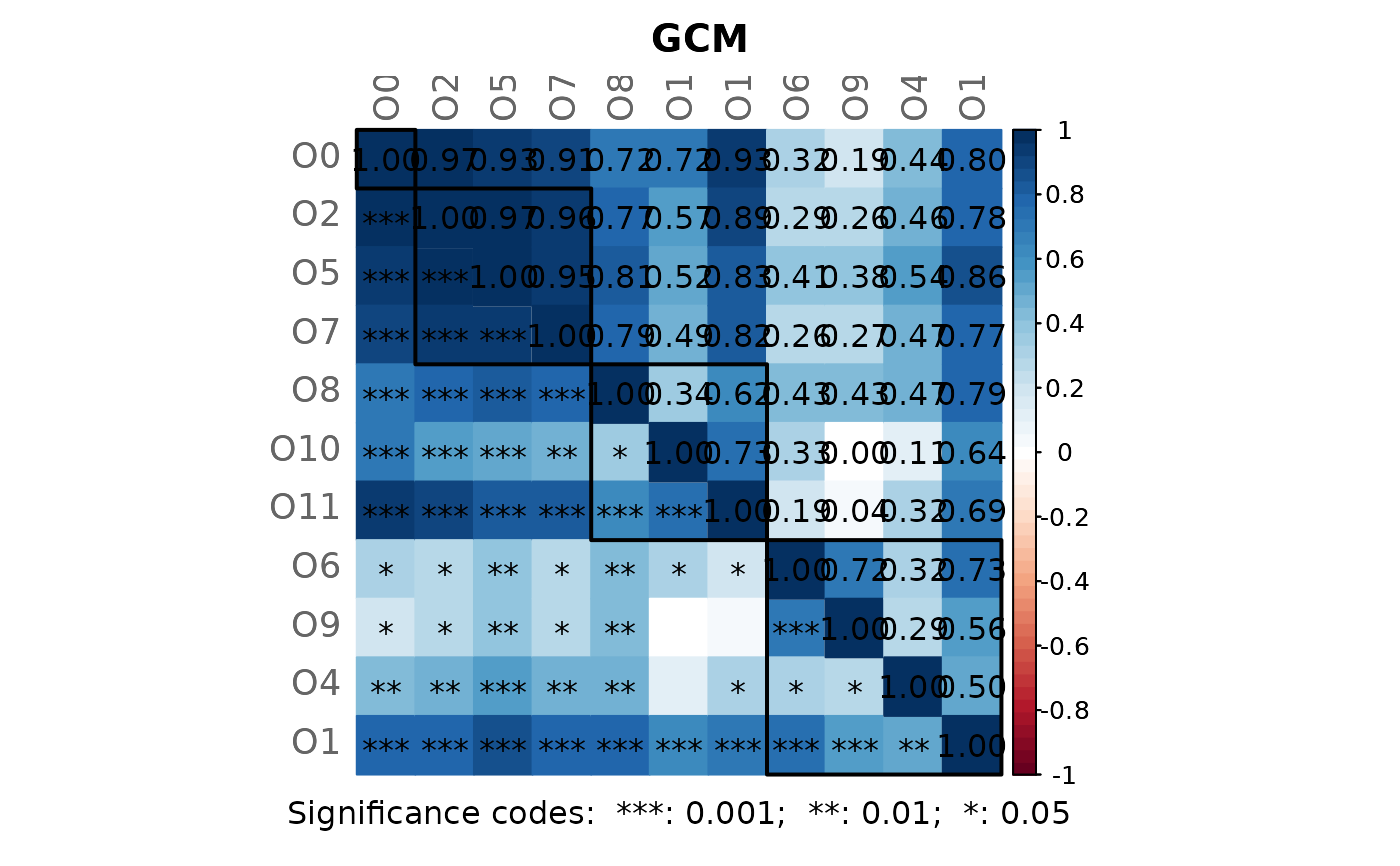
graphlet: logical. If TRUE (default), graphlet-based network properties are computed: orbit counts as defined by orbits and the corresponding Graphlet Correlation Matrix (gcm).
orbits: numeric vector with integers from 0 to 14 defining the orbits used for calculating the GCM. Minimum length is 2. Defaults to c(0, 1, 2, 4, 5, 6, 7, 8, 9, 10, 11), thus excluding redundant orbits such as the orbit o3.
gcmHeat: logical indicating if a heatmap of the GCM(s) should be plotted. Default is TRUE.
gcmHeatLCC: logical. The GCM heatmap is plotted for the LCC if TRUE (default) and for the whole network if FALSE.
avDissIgnoreInf: logical indicating whether to ignore infinities when calculating the average dissimilarity. If FALSE (default), infinity values are set to 1.
sPathAlgo: character indicating the algorithm used for computing the shortest paths between all node pairs. distances (igraph) is used for shortest path calculation. Possible values are: "unweighted", "dijkstra" (default), "bellman-ford", "johnson", or "automatic" (the fastest suitable algorithm is used). The shortest paths are needed for the average (shortest) path length and closeness centrality.
sPathNorm: logical. If TRUE (default), shortest paths are normalized by average dissimilarity (only connected nodes are considered), i.e., a path is interpreted as steps with average dissimilarity. If FALSE, the shortest path is the minimum sum of dissimilarities between two nodes.
normNatConnect: logical. If TRUE (default), the normalized natural connectivity is returned.
connectivity: logical. If TRUE (default), edge and vertex connectivity are calculated. Might be disabled to reduce execution time.
verbose: integer indicating the level of verbosity. Possible values: "0": no messages, "1": only important messages, "2"(default): all progress messages are shown. Can also be logical.

Value

An object of class microNetProps containing the following elements:

`lccNames1, lccNames2`	Names of nodes in the largest connected component(s).
`compSize1, compSize2`	Matrix/matrices with component sizes (1st row: sizes; 2nd row: number of components with the respective size)
`clustering`	Determined clusters in the whole network (and corresponding trees if hierarchical clustering is used)
`clusteringLCC`	Clusters (and optional trees) of the largest connected component.
`centralities`	Centrality values
`hubs`	Names of hub nodes
`globalProps`	Global network properties of the whole network.
`globalPropsLCC`	Global network properties of the largest component.
`graphlet`	Graphlet-based properties (orbit counts and GCM).
`graphletLCC`	Graphlet-based properties of the largest connected component.
`paramsProperties`	Given parameters used for network analysis
`paramsNetConstruct`	Parameters used for network construction (inherited from `netConstruct`).
`input`	Input inherited from `netConstruct`.
`isempty`	Indicates whether network(s) is/are empty.

Details

Definitions:

(Connected) Component: Subnetwork where any two nodes are connected by a path.
Number of components: Number of connected components. Since a single node is connected to itself by the trivial path, each single node is a component.
Largest connected component (LCC): The connected component with highest number of nodes.
Shortest paths: Computed using distances. The algorithm is defined via sPathAlgo. Normalized shortest paths (if sPathNorm is TRUE) are calculated by dividing the shortest paths by the average dissimilarity (see below).

Global network properties:

Relative LCC size: = (# nodes in the LCC) / (# nodes in the complete network)
Clustering Coefficient: The weighted (global) clustering coefficient is the arithmetic mean of the local clustering coefficient defined by Barrat et al. (computed by transitivity with type = "barrat"), where NAs are ignored.
The unweighted (global) clustering coefficient is computed using transitivity with type = "global".
Modularity: The modularity score for the determined clustering is computed using modularity.igraph.
Positive edge percentage: Percentage of edges with positive estimated association of the total number of edges.
Edge density: Computed using edge_density.
Natural connectivity: Computed using natural.connectivity. The "norm" parameter is defined by normNatConnect.
Vertex / Edge connectivity: Computed using vertex_connectivity and edge_connectivity. Both equal zero for a disconnected network.
Average dissimilarity: Computed as the mean of dissimilarity values (lower triangle of dissMat). By avDissIgnoreInf is specified whether to ignore infinite dissimilarities. The average dissimilarity of an empty network is 1.
Average path length: Computed as the mean of shortest paths (normalized or unnormalized). The av. path length of an empty network is 1.

Clustering algorithms:

Hierarchical clustering: Based on dissimilarity values. Computed using hclust and cutree.
cluster_optimal: Modularity optimization. See cluster_optimal.
cluster_fast_greedy: Fast greedy modularity optimization. See cluster_fast_greedy.
cluster_louvain: Multilevel optimization of modularity. See cluster_louvain.
cluster_edge_betweenness: Based on edge betweenness. Dissimilarity values are used. See cluster_edge_betweenness.
cluster_leading_eigen: Based on leading eigenvector of the community matrix. See cluster_leading_eigen.
cluster_spinglass: Find communities via spin-glass model and simulated annealing. See cluster_spinglass.
cluster_walktrap: Find communities via short random walks. See cluster_walktrap.

Hubs:
Hubs are nodes with highest centrality values for one or more centrality measures. The "highest values" regarding a centrality measure are defined as values lying above a certain quantile (defined by hubQuant) either of the empirical distribution of the centralities (if lnormFit = FALSE) or of the fitted log-normal distribution (if lnormFit = TRUE; fitdistr is used for fitting). The quantile is set using hubQuant.
If clustPar contains multiple measures, the centrality values of a hub node must be above the given quantile for all measures at the same time.

Centrality measures:
Via centrLCC is decided whether centralities should be calculated for the whole network or only for the largest connected component. In the latter case (centrLCC = FALSE), nodes outside the LCC have a centrality value of zero.

Degree: The unweighted degree (normalized and unnormalized) is computed using degree, and the weighted degree using strength.
Betweenness centrality: The unnormalized and normalized betweenness centrality is computed using betweenness.
Closeness centrality: Unnormalized: closeness = sum(1/shortest paths)
Normalized: closeness_unnorm = closeness / (# nodes – 1)
Eigenvector centrality: If centrLCC == FALSE and the network consists of more than one components: The eigenvector centrality (EVC) is computed for each component separately (using eigen_centrality) and scaled according to component size to overcome the fact that nodes in smaller components have a higher EVC. If normEigen == TRUE, the EVC values are divided by the maximum EVC value. EVC of single nodes is zero.

Otherwise, the EVC is computed for the LCC using eigen_centrality (scale argument is set according to normEigen).

Graphlet-based properties:

Orbit counts: Count of node orbits in graphlets with 2 to 4 nodes. See Hocevar and Demsar (2016) for details. The count4 function from orca package is used for orbit counting.
Graphlet Correlation Matrix (GCM): Matrix with Spearman's correlations between the network's (non-redundant) node orbits (Yaveroglu et al., 2014).

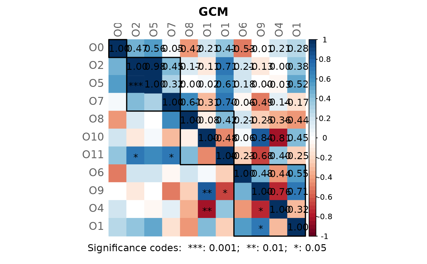
By default, only the 11 non-redundant orbits are used. These are grouped according to their role: orbit 0 represents the degree, orbits (2, 5, 7) represent nodes within a chain, orbits (8, 10, 11) represent nodes in a cycle, and orbits (6, 9, 4, 1) represent a terminal node.

References

hocevar2016computationNetCoMi

yaveroglu2014revealingNetCoMi

Examples

# Load data sets from American Gut Project (from SpiecEasi package)
data("amgut1.filt")

# Network construction
amgut_net1 <- netConstruct(amgut1.filt, measure = "pearson",
                           filtTax = "highestVar",
                           filtTaxPar = list(highestVar = 50),
                           zeroMethod = "pseudoZO", normMethod = "clr",
                           sparsMethod = "threshold", thresh = 0.4)
#> Checking input arguments ... 
#> Done.
#> Data filtering ...
#> 77 taxa removed.
#> 50 taxa and 289 samples remaining.
#> 
#> Zero treatment:
#> Zero counts replaced by 1
#> 
#> Normalization:
#> Execute clr(){SpiecEasi} ... 
#> Done.
#> 
#> Calculate 'pearson' associations ... 
#> Done.
#> 
#> Sparsify associations via 'threshold' ... 
#> Done.

# Network analysis

# Using eigenvector centrality as hub score
amgut_props1 <- netAnalyze(amgut_net1, clustMethod = "cluster_fast_greedy",
                           hubPar = "eigenvector")

                           
summary(amgut_props1, showCentr = "eigenvector", numbNodes = 15L, digits = 3L)
#> 
#> Component sizes
#> ```````````````               
#> size: 12 6 2  1
#>    #:  1 1 1 30
#> ______________________________
#> Global network properties
#> `````````````````````````
#> Largest connected component (LCC):
#>                                
#> Relative LCC size         0.240
#> Clustering coefficient    0.733
#> Modularity                0.338
#> Positive edge percentage 86.364
#> Edge density              0.333
#> Natural connectivity      0.190
#> Vertex connectivity       1.000
#> Edge connectivity         1.000
#> Average dissimilarity*    0.820
#> Average path length**     1.526
#> 
#> Whole network:
#>                                
#> Number of components     33.000
#> Clustering coefficient    0.523
#> Modularity                0.512
#> Positive edge percentage 89.286
#> Edge density              0.023
#> Natural connectivity      0.028
#> -----
#> *: Dissimilarity = 1 - edge weight
#> **: Path length = Units with average dissimilarity
#> 
#> ______________________________
#> Clusters
#> - In the whole network
#> - Algorithm: cluster_fast_greedy
#> ```````````````````````````````` 
#>                   
#> name:  0 1 2 3 4 5
#>    #: 30 6 4 2 5 3
#> 
#> ______________________________
#> Hubs
#> - In alphabetical/numerical order
#> - Based on empirical quantiles of centralities
#> ```````````````````````````````````````````````       
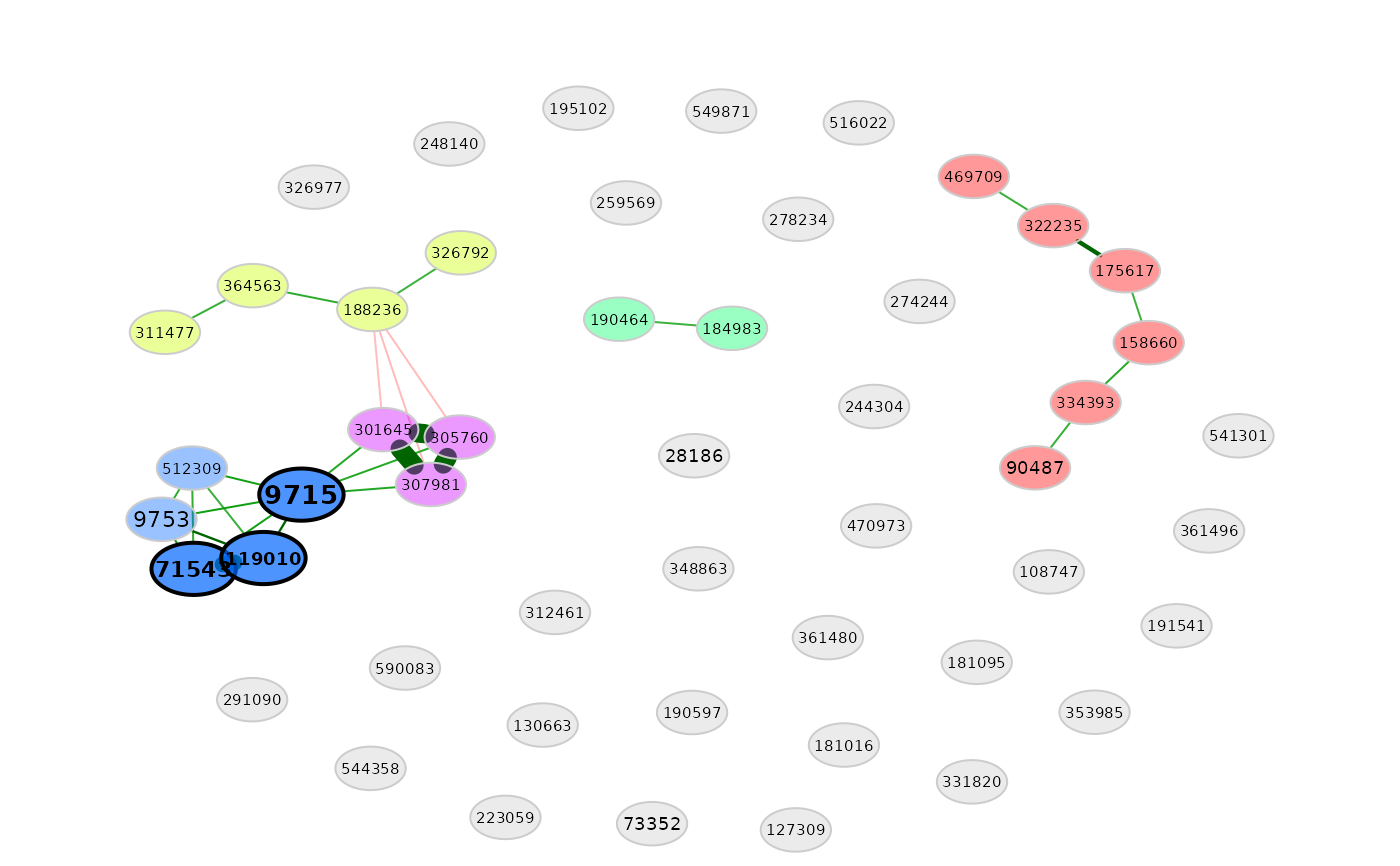
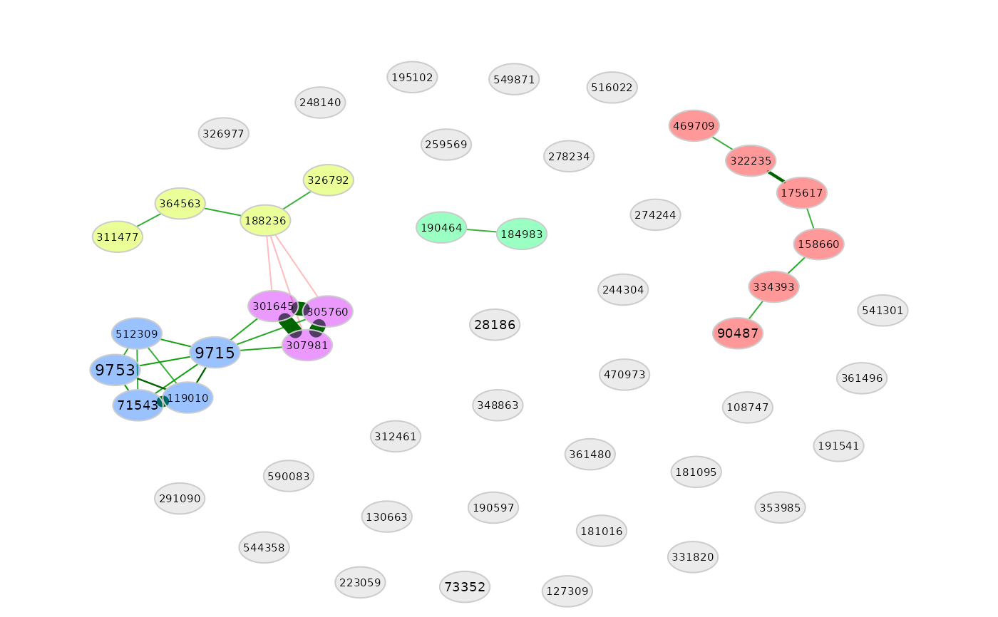
#>  119010
#>  71543 
#>  9715  
#> 
#> ______________________________
#> Centrality measures
#> - In decreasing order
#> - Centrality of disconnected components is zero
#> ````````````````````````````````````````````````
#> Eigenvector centrality (normalized):
#>             
#> 9715   1.000
#> 119010 0.733
#> 71543  0.723
#> 9753   0.670
#> 307981 0.670
#> 301645 0.670
#> 305760 0.669
#> 512309 0.607
#> 188236 0.131
#> 364563 0.026
#> 326792 0.023
#> 311477 0.005
#> 73352  0.000
#> 331820 0.000
#> 248140 0.000

# Using degree, betweenness and closeness centrality as hub scores
amgut_props2 <- netAnalyze(amgut_net1, clustMethod = "cluster_fast_greedy",
                           hubPar = c("degree", "betweenness", "closeness"))

summary(amgut_props2, showCentr = "all",  numbNodes = 5L, digits = 5L)
#> 
#> Component sizes
#> ```````````````               
#> size: 12 6 2  1
#>    #:  1 1 1 30
#> ______________________________
#> Global network properties
#> `````````````````````````
#> Largest connected component (LCC):
#>                                  
#> Relative LCC size         0.24000
#> Clustering coefficient    0.73277
#> Modularity                0.33781
#> Positive edge percentage 86.36364
#> Edge density              0.33333
#> Natural connectivity      0.19028
#> Vertex connectivity       1.00000
#> Edge connectivity         1.00000
#> Average dissimilarity*    0.82023
#> Average path length**     1.52564
#> 
#> Whole network:
#>                                  
#> Number of components     33.00000
#> Clustering coefficient    0.52341
#> Modularity                0.51212
#> Positive edge percentage 89.28571
#> Edge density              0.02286
#> Natural connectivity      0.02791
#> -----
#> *: Dissimilarity = 1 - edge weight
#> **: Path length = Units with average dissimilarity
#> 
#> ______________________________
#> Clusters
#> - In the whole network
#> - Algorithm: cluster_fast_greedy
#> ```````````````````````````````` 
#>                   
#> name:  0 1 2 3 4 5
#>    #: 30 6 4 2 5 3
#> 
#> ______________________________
#> Hubs
#> - In alphabetical/numerical order
#> - Based on empirical quantiles of centralities
#> ```````````````````````````````````````````````
#> No hubs detected.
#> ______________________________
#> Centrality measures
#> - In decreasing order
#> - Centrality of disconnected components is zero
#> ````````````````````````````````````````````````
#> Degree (normalized):
#>               
#> 9715   0.14286
#> 188236 0.10204
#> 307981 0.08163
#> 71543  0.08163
#> 512309 0.08163
#> 
#> Betweenness centrality (normalized):
#>               
#> 9715   0.50909
#> 188236 0.47273
#> 307981 0.36364
#> 364563 0.18182
#> 73352  0.00000
#> 
#> Closeness centrality (normalized):
#>               
#> 305760 2.17422
#> 301645 2.13487
#> 307981 2.12892
#> 119010 1.36913
#> 71543  1.33707
#> 
#> Eigenvector centrality (normalized):
#>               
#> 9715   1.00000
#> 119010 0.73317
#> 71543  0.72255
#> 9753   0.67031
#> 307981 0.67026

# Calculate centralities only for the largest connected component
amgut_props3 <- netAnalyze(amgut_net1, centrLCC = TRUE, 
                           clustMethod = "cluster_fast_greedy",
                           hubPar = "eigenvector")

summary(amgut_props3, showCentr = "none", clusterLCC = TRUE)
#> 
#> Component sizes
#> ```````````````               
#> size: 12 6 2  1
#>    #:  1 1 1 30
#> ______________________________
#> Global network properties
#> `````````````````````````
#> Largest connected component (LCC):
#>                                  
#> Relative LCC size         0.24000
#> Clustering coefficient    0.73277
#> Modularity                0.33781
#> Positive edge percentage 86.36364
#> Edge density              0.33333
#> Natural connectivity      0.19028
#> Vertex connectivity       1.00000
#> Edge connectivity         1.00000
#> Average dissimilarity*    0.82023
#> Average path length**     1.52564
#> 
#> Whole network:
#>                                  
#> Number of components     33.00000
#> Clustering coefficient    0.52341
#> Modularity                0.51212
#> Positive edge percentage 89.28571
#> Edge density              0.02286
#> Natural connectivity      0.02791
#> -----
#> *: Dissimilarity = 1 - edge weight
#> **: Path length = Units with average dissimilarity
#> 
#> ______________________________
#> Clusters
#> - In the LCC
#> - Algorithm: cluster_fast_greedy
#> ```````````````````````````````` 
#>            
#> name: 1 2 3
#>    #: 4 5 3
#> 
#> ______________________________
#> Hubs
#> - In alphabetical/numerical order
#> - Based on empirical quantiles of centralities
#> ```````````````````````````````````````````````       
#>  119010
#>  71543 
#>  9715  

# Network plot
plot(amgut_props1)

plot(amgut_props2)

plot(amgut_props3)


#----------------------------------------------------------------------------
# Plot the GCM heatmap
plotHeat(mat = amgut_props1$graphletLCC$gcm1,
         pmat = amgut_props1$graphletLCC$pAdjust1,
         type = "mixed",
         title = "GCM", 
         colorLim = c(-1, 1),
         mar = c(2, 0, 2, 0))
# Add rectangles
graphics::rect(xleft   = c( 0.5,  1.5, 4.5,  7.5),
               ybottom = c(11.5,  7.5, 4.5,  0.5),
               xright  = c( 1.5,  4.5, 7.5, 11.5),
               ytop    = c(10.5, 10.5, 7.5,  4.5),
               lwd = 2, xpd = NA)

text(6, -0.2, xpd = NA, 
     "Significance codes:  ***: 0.001;  **: 0.01;  *: 0.05")


#----------------------------------------------------------------------------
# Dissimilarity-based network (where nodes are subjects)
amgut_net4 <- netConstruct(amgut1.filt, measure = "aitchison",
                           filtSamp = "highestFreq",
                           filtSampPar = list(highestFreq = 30),
                           zeroMethod = "multRepl", sparsMethod = "knn")
#> Checking input arguments ... 
#> Done.
#> Infos about changed arguments:
#> Counts normalized to fractions for measure "aitchison".
#> Data filtering ...
#> 259 samples removed.
#> 127 taxa and 30 samples remaining.
#> 
#> Zero treatment:
#> Execute multRepl() ... 
#> Done.
#> 
#> Normalization:
#> Counts normalized by total sum scaling.
#> 
#> Calculate 'aitchison' dissimilarities ... 
#> Done.
#> 
#> Sparsify dissimilarities via 'knn' ... 
#> Done.

amgut_props4 <- netAnalyze(amgut_net4, clustMethod = "hierarchical",
                           clustPar = list(k = 3))


plot(amgut_props4)