Construct microbial association networks and dissimilarity-based networks (where nodes are subjects) from compositional count data.
Usage
netConstruct(data,
             data2 = NULL,
             dataType = "counts",
             group = NULL,
             matchDesign = NULL,
             taxRank = NULL,

             # Association/dissimilarity measure:
             measure = "spieceasi",
             measurePar = NULL,

             # Preprocessing:
             jointPrepro = NULL,
             filtTax = "none",
             filtTaxPar = NULL,
             filtSamp = "none",
             filtSampPar = NULL,
             zeroMethod = "none",
             zeroPar = NULL,
             normMethod = "none",
             normPar = NULL,

             # Sparsification:
             sparsMethod = "t-test",
             thresh = 0.3,
             alpha = 0.05,
             adjust = "adaptBH",
             trueNullMethod = "convest",
             lfdrThresh = 0.2,
             nboot = 1000L,
             assoBoot = NULL,
             cores = 1L,
             logFile = "log.txt",
             softThreshType = "signed",
             softThreshPower = NULL,
             softThreshCut = 0.8,
             kNeighbor = 3L,
             knnMutual = FALSE,

             # Transformation:
             dissFunc = "signed",
             dissFuncPar = NULL,
             simFunc = NULL,
             simFuncPar = NULL,
             scaleDiss = TRUE,
             weighted = TRUE,

             # Further arguments:
             sampleSize = NULL,
             verbose = 2,
             seed = NULL
             )
Arguments
- data
data set from which the network is built. Can be a numeric matrix (samples in rows, OTUs/ASVs in columns) or an object of the classes:
phyloseq,SummarizedExperiment,TreeSummarizedExperiment. Can also be an association or dissimilarity matrix (dataTypemust be set accordingly).- data2
optional data set for constructing a second network (belonging to group 2). Accepted input is the same as for
data.- dataType
character indicating the data type. Defaults to "counts", which means that
data(and data2) is a count matrix or object of classphyloseq,SummarizedExperiment, orTreeSummarizedExperiment. Further options are "association", "correlation", "partialCorr" (partial correlation), "condDependence" (conditional dependence), "proportionality", and "dissimilarity".- group
optional binary vector used for splitting the data into two groups. If
groupisNULL(default) anddata2is not set, a single network is constructed. See 'Details.'- matchDesign
Numeric vector with two elements specifying an optional matched-group (i.e. matched-pair) design, which is used for the permutation tests in
netCompareanddiffnet.c(1,1)corresponds to a matched-pair design. A 1:2 matching, for instance, is defined byc(1,2), which means that the first sample of group 1 is matched to the first two samples of group 2 and so on. The appropriate order of samples must be ensured. IfNULL, the group memberships are shuffled randomly while group sizes identical to the original data set are ensured.- taxRank
character indicating the taxonomic rank at which the network should be constructed. Only used if data (and data 2) is a phyloseq object. The given rank must match one of the column names of the taxonomy table (the
@tax_tableslot of the phyloseq object). Taxa names of the chosen taxonomic rank must be unique (consider using the functionrenameTaxato make them unique). If a phyloseq object is given andtaxRank = NULL, the row names of the OTU table are used as node labels.- measure
character specifying the method used for either computing the associations between taxa or dissimilarities between subjects. Ignored if
datais not a count matrix (ifdataTypeis not set to"counts"). Available measures are:"pearson","spearman","bicor","sparcc","cclasso","ccrepe","spieceasi"(default),"spring","gcoda"and"propr"as association measures, and"euclidean","bray","kld","jeffrey","jsd","ckld", and"aitchison"as dissimilarity measures. Parameters are set viameasurePar.- measurePar
list with parameters passed to the function for computing associations/dissimilarities. See 'Details' for the respective functions. For SpiecEasi or SPRING as association measure, an additional list element "symBetaMode" is accepted to define the "mode" argument of
symBeta.- jointPrepro
logical indicating whether data preprocessing (filtering, zero treatment, normalization) should be done for the combined data sets, or each data set separately. Ignored if a single network is constructed. Defaults to
TRUEifgroupis given, and toFALSEifdata2is given. Joint preprocessing is not possible for dissimilarity networks.- filtTax
character indicating how taxa shall be filtered. Possible options are:
"none"Default. All taxa are kept.
"totalReads"Keep taxa with a total number of reads of at least x.
"relFreq"Keep taxa whose number of reads is at least x% of the total number of reads.
"numbSamp"Keep taxa observed in at least x samples.
"highestVar"Keep the x taxa with highest variance.
"highestFreq"Keep the x taxa with highest frequency.
Except for "highestVar" and "highestFreq", different filter methods can be combined. The values x are set via
filtTaxPar.- filtTaxPar
list with parameters for the filter methods given by
filtTax. Possible list entries are:"totalReads"(int),"relFreq"(value in [0,1]),"numbSamp"(int),"highestVar"(int),"highestFreq"(int).- filtSamp
character indicating how samples shall be filtered. Possible options are:
"none"Default. All samples are kept.
"totalReads"Keep samples with a total number of reads of at least x.
"numbTaxa"Keep samples for which at least x taxa are observed.
"highestFreq"Keep the x samples with highest frequency.
Except for "highestFreq", different filter methods can be combined. The values x are set via
filtSampPar.- filtSampPar
list with parameters for the filter methods given by
filtSamp. Possible list entries are:"totalReads"(int),"numbTaxa"(int),"highestFreq"(int).- zeroMethod
character indicating the method used for zero replacement. Possible values are:
"none"(default),"pseudo","pseudoZO","multRepl","alrEM","bayesMult". See 'Details'. The corresponding parameters are set viazeroPar.zeroMethodis ignored if the approach for calculating the associations/dissimilarity includes zero handling. Defaults to"multRepl"or"pseudo"(depending on the expected input of the normalization function and measure) if zero replacement is required.- zeroPar
list with parameters passed to the function for zero replacement (
zeroMethod). See the help page of the respective function for details. IfzeroMethodis"pseudo"or"pseudoZO", the pseudo count can be specified viazeroPar = list(pseudocount = x)(where x is numeric).- normMethod
character indicating the normalization method (to make counts of different samples comparable). Possible options are:
"none"(default),"TSS"(or"fractions"),"CSS","COM","rarefy","VST","clr", and"mclr". See 'Details'. The corresponding parameters are set vianormPar.- normPar
list with parameters passed to the function for normalization (defined by
normMethod).- sparsMethod
character indicating the method used for sparsification (selected edges that are connected in the network). Available methods are:
"none"Leads to a fully connected network
"t-test"Default. Associations being significantly different from zero are selected using Student's t-test. Significance level and multiple testing adjustment is specified via
alphaandadjust.sampleSizemust be set ifdataTypeis not "counts"."bootstrap"Bootstrap procedure as described in Friedman and Alm (2012). Corresponding arguments are
nboot,cores, andlogFile. Data type must be "counts"."threshold"Selected are taxa pairs with an absolute association/dissimilarity greater than or equal to the threshold defined via
thresh."softThreshold"Soft thresholding method according to Zhang and Horvath (2005) available in the
WGCNApackage. Corresponding arguments aresoftThreshType,softThreshPower, andsoftThreshCut."knn"Construct a k-nearest neighbor or mutual k-nearest neighbor graph using
nng. Corresponding arguments arekNeighbor, andknnMutual. Available for dissimilarity networks only.
- thresh
numeric vector with one or two elements defining the threshold used for sparsification if
sparsMethodis set to"threshold". If two networks are constructed and one value is given, it is used for both groups. Defaults to 0.3.- alpha
numeric vector with one or two elements indicating the significance level. Only used if Student's t-test or bootstrap procedure is used as sparsification method. If two networks are constructed and one value is given, it is used for both groups. Defaults to 0.05.
- adjust
character indicating the method used for multiple testing adjustment (if Student's t-test or bootstrap procedure is used for edge selection). Possible values are
"lfdr"(default) for local false discovery rate correction (viafdrtool),"adaptBH"for the adaptive Benjamini-Hochberg method (Benjamini and Hochberg, 2000), or one of the methods provided byp.adjust(seep.adjust.methods().- trueNullMethod
character indicating the method used for estimating the proportion of true null hypotheses from a vector of p-values. Used for the adaptive Benjamini-Hochberg method for multiple testing adjustment (chosen by
adjust = "adaptBH"). Accepts the provided options of themethodargument ofpropTrueNull:"convest"(default),"lfdr","mean", and"hist". Can alternatively be"farco"for the "iterative plug-in method" proposed by Farcomeni (2007).- lfdrThresh
numeric vector with one or two elements defining the threshold(s) for local FDR correction (if
adjust = "locfdr"). Defaults to 0.2 meaning that associations with a corresponding local FDR less than or equal to 0.2 are identified as significant. If two networks are constructed and one value is given, it is used for both groups.- nboot
integer indicating the number of bootstrap samples, if bootstrapping is used as sparsification method.
- assoBoot
logical or list. Only relevant for bootstrapping. Set to
TRUEif a list (assoBoot) with bootstrap association matrices should be returned. Can also be a list with bootstrap association matrices, which are used for sparsification. See the example.- cores
integer indicating the number of CPU cores used for bootstrapping. If cores > 1, bootstrapping is performed parallel.
coresis limited to the number of available CPU cores determined bydetectCores. Then, core arguments of the function used for association estimation (if provided) should be set to 1.- logFile
character defining a log file to which the iteration numbers are stored if bootstrapping is used for sparsification. The file is written to the current working directory. Defaults to
"log.txt". IfNULL, no log file is created.- softThreshType
character indicating the method used for transforming correlations into similarities if soft thresholding is used as sparsification method (
sparsMethod = "softThreshold"). Possible values are"signed","unsigned", and"signed hybrid"(according to the available options for the argumenttypeofadjacencyfromWGCNApackage).- softThreshPower
numeric vector with one or two elements defining the power for soft thresholding. Only used if
edgeSelect = "softThreshold". If two networks are constructed and one value is given, it is used for both groups. If no power is set, it is computed usingpickSoftThreshold, where the argumentsoftThreshCutis needed in addition.- softThreshCut
numeric vector with one or two elements (each between 0 and 1) indicating the desired minimum scale free topology fitting index (corresponds to the argument "RsquaredCut" in
pickSoftThreshold). Defaults to 0.8. If two networks are constructed and one value is given, it is used for both groups.- kNeighbor
integer specifying the number of neighbors if the k-nearest neighbor method is used for sparsification. Defaults to 3L.
- knnMutual
logical used for k-nearest neighbor sparsification. If
TRUE, the neighbors must be mutual. Defaults toFALSE.- dissFunc
method used for transforming associations into dissimilarities. Can be a character with one of the following values:
"signed"(default),"unsigned","signedPos","TOMdiss". Alternatively, a function is accepted with the association matrix as first argument and optional further arguments, which can be set viadissFuncPar. Ignored for dissimilarity measures. See 'Details.'- dissFuncPar
optional list with parameters if a function is passed to
dissFunc.- simFunc
function for transforming dissimilarities into similarities. Defaults to f(x)=1-x for dissimilarities in [0,1], and f(x)=1/(1 + x) otherwise.
- simFuncPar
optional list with parameters for the function passed to
simFunc.- scaleDiss
logical. Indicates whether dissimilarity values should be scaled to [0,1] by (x - min(dissEst)) / (max(dissEst) - min(dissEst)), where dissEst is the matrix with estimated dissimilarities. Defaults to
TRUE.- weighted
logical. If
TRUE, similarity values are used as adjacencies.FALSEleads to a binary adjacency matrix whose entries equal 1 for (sparsified) similarity values > 0, and 0 otherwise.- sampleSize
numeric vector with one or two elements giving the number of samples that have been used for computing the association matrix. Only needed if an association matrix is given instead of a count matrix and if, in addition, Student's t-test is used for edge selection. If two networks are constructed and one value is given, it is used for both groups.
- verbose
integer indicating the level of verbosity. Possible values:
"0": no messages,"1": only important messages,"2"(default): all progress messages,"3"messages returned by external functions are shown in addition. Can also be logical.- seed
integer giving a seed for reproducibility of the results.
Value
An object of class microNet containing the following elements:
edgelist1, edgelist2 | Edge list with the following columns:
|
assoMat1, assoMat2 | Sparsified associations (NULL for
dissimilarity based networks) |
dissMat1, dissMat2 | Sparsified dissimilarities (for association networks, these are the sparsified associations transformed into dissimilarities) |
simMat1, simMat2 | Sparsified similarities |
adjaMat1, adjaMat2 | Adjacency matrices |
assoEst1, assoEst2 | Estimated associations (NULL for
dissimilarity based networks) |
dissEst1, dissEst2 | Estimated dissimilarities (NULL for
association networks) |
dissScale1, dissScale2 | Scaled dissimilarities (NULL for
association networks) |
assoBoot1, assoBoot2 | List with association matrices for the
bootstrap samples. Returned if bootstrapping is used for
sparsification and assoBoot is TRUE. |
countMat1, countMat2 | Count matrices after filtering but before
zero replacement and normalization. Only returned if jointPrepro
is FALSE or for a single network. |
countsJoint | Joint count matrix after filtering but before
zero replacement and normalization. Only returned if jointPrepro
is TRUE. |
normCounts1, normCounts2 | Count matrices after zero handling and normalization |
measureOut1, measureOut2 | Output returned by the function used for association or dissimilarity estimation (defined via `measure`). |
groups | Names of the factor levels according to which the groups have been built |
softThreshPower | Determined (or given) power for soft-thresholding. |
assoType | Data type (either given by dataType or
determined from measure) |
twoNets | Indicates whether two networks have been constructed |
parameters | Parameters used for network construction |
Details
The object returned by netConstruct can either be passed to
netAnalyze for network analysis, or to
diffnet to construct a differential network from the
estimated associations.
The function enables the construction of either a single network
or two networks. The latter can be compared using the function
netCompare.
The network(s) can either be based on associations (correlation,
partial correlation / conditional dependence, proportionality) or
dissimilarities. Several measures are available, respectively,
to estimate associations or dissimilarities using netConstruct.
Alternatively, a pre-generated association or dissimilarity matrix is
accepted as input to start the workflow (argument dataType must be
set appropriately).
Depending on the measure, network nodes are either taxa or subjects:
In association-based networks nodes are taxa, whereas in
dissimilarity-based networks nodes are subjects.
In order to perform a network comparison, the following options
for constructing two networks are available:
Passing the combined count matrix to
dataand a group vector togroup(of lengthnrow(data)for association networks and of lengthncol(data)for dissimilarity-based networks).Passing the count data for group 1 to
data(matrix or phyloseq object) and the count data for group 2 todata2(matrix or phyloseq object). For association networks, the column names must match, and for dissimilarity networks the row names.Passing an association/dissimilarity matrix for group 1 to
dataand an association/dissimilarity matrix for group 2 todata2.
Group labeling:
If two networks are generated, the network belonging to data
is always denoted by "group 1" and the network belonging to data2
by "group 2".
If a group vector is used for splitting the data into two groups, the group
names are assigned according to the order of group levels. If group
contains the levels 0 and 1, for instance, "group 1" is assigned to level 0
and "group 2" is assigned to level 1.
In the network plot, group 1 is shown on the left and group 2 on the
right if not defined otherwise (see plot.microNetProps).
Association measures
| Argument | Function |
"pearson" | cor |
"spearman" | cor |
"bicor" | bicor |
"sparcc" | sparcc |
"cclasso" | cclasso |
"ccrepe" | ccrepe |
"spieceasi" | spiec.easi |
"spring" | SPRING |
"gcoda" | gcoda |
"propr" | propr |
Dissimilarity measures
| Argument | Function | Measure |
"euclidean" | vegdist | Euclidean distance |
"bray" | vegdist | Bray-Curtis dissimilarity |
"kld" | KLD | Kullback-Leibler divergence |
"jeffrey" | KLD | Jeffrey divergence |
"jsd" | KLD | Jensen-Shannon divergence |
"ckld" | log | Compositional Kullback-Leibler divergence |
"aitchison" | vegdist,
cenLR | Aitchison distance |
Definitions:
- Kullback-Leibler divergence:
Since KLD is not symmetric, 0.5 * (KLD(p(x)||p(y)) + KLD(p(y)||p(x))) is returned.
- Jeffrey divergence:
Jeff = KLD(p(x)||p(y)) + KLD(p(y)||p(x))
- Jensen-Shannon divergence:
JSD = 0.5 KLD(P||M) + 0.5 KLD(Q||M), where P=p(x), Q=p(y), and M=0.5(P+Q).
- Compositional Kullback-Leibler divergence:
cKLD(x,y) = p/2 * log(A(x/y) * A(y/x)), where A(x/y) is the arithmetic mean of the vector of ratios x/y.
- Aitchison distance:
Euclidean distance of the clr-transformed data.
Methods for zero replacement
| Argument | Method | Function |
"none" | No zero replacement (only available if no zero replacement is needed for the chosen normalization method and association/dissimilarity measure). | - |
"pseudo" | A pseudo count (defined by pseudocount as
optional element of zeroPar) is added to all counts. A unit zero
count is used by default. | - |
"pseudoZO" | A pseudo count (defined by pseudocount as
optional element of zeroPar) is added to zero counts only.
A unit zero count is used by default. | - |
"multRepl" | Multiplicative simple replacement | multRepl |
"alrEM" | Modified EM alr-algorithm | lrEM |
"bayesMult" | Bayesian-multiplicative replacement | cmultRepl |
Normalization methods
| Argument | Method | Function |
"TSS" | Total sum scaling | t(apply(countMat, 1, function(x) x/sum(x))) |
"CSS" | Cumulative sum scaling | cumNormMat |
"COM" | Common sum scaling | t(apply(countMat, 1, function(x) x * min(rowSums(countMat)) / sum(x))) |
"rarefy" | Rarefying | rrarefy |
"VST" | Variance stabilizing transformation | varianceStabilizingTransformation |
"clr" | Centered log-ratio transformation | clr |
"mclr" | Modified central log ratio transformation | mclr |
These methods (except for rarefying) are described in
Badri et al.(2020).
Transformation methods
Functions used for transforming associations into dissimilarities:
| Argument | Function |
"signed" | sqrt(0.5 * (1 - x)) |
"unsigned" | sqrt(1 - x^2) |
"signedPos" | diss <- sqrt(0.5 * (1-x)) |
| diss[x < 0] <- 0 | |
"TOMdiss" | TOMdist |
References
Badri M, Kurtz ZD, Bonneau R, Mueller CL (2020). “Shrinkage improves
estimation of microbial associations under different normalization methods.”
NAR Genomics and Bioinformatics, 2(4).
Benjamini Y, Hochberg Y (2000). “On the adaptive control of the false
discovery rate in multiple testing with independent statistics.”
Journal of Educational and Behavioral Statistics, 25(1), 60–83.
Farcomeni A (2007). “Some results on the control of the false discovery rate
under dependence.” Scandinavian Journal of Statistics, 34(2),
275–297.
Friedman J, Alm EJ (2012). “Inferring Correlation Networks from Genomic
Survey Data.” PLoS Computational Biology, 8, e1002687.
Langfelder P, Horvath S (2008). “WGCNA: an R package for weighted
correlation network analysis.” BMC Bioinformatics, 9(1), 559.
Zhang B, Horvath S (2005). “A General Framework for Weighted Gene
Co-Expression Network Analysis.”
Statistical Applications in Genetics and Molecular Biology, 4, 17.
See also
netAnalyze for analyzing the constructed
network(s), netCompare for network comparison,
diffnet for constructing differential networks.
Examples
knitr::opts_chunk$set(fig.width = 8, fig.height = 8)
# Load data sets from American Gut Project (from SpiecEasi package)
data("amgut1.filt")
data("amgut2.filt.phy")
# Single network with the following specifications:
# - Association measure: SpiecEasi
# - SpiecEasi parameters are defined via 'measurePar'
# (check ?SpiecEasi::spiec.easi for available options)
# - Note: 'rep.num' should be higher for real data sets
# - Taxa filtering: Keep the 50 taxa with highest variance
# - Sample filtering: Keep samples with a total number of reads
# of at least 1000
net1 <- netConstruct(amgut2.filt.phy,
measure = "spieceasi",
measurePar = list(method = "mb",
pulsar.params = list(rep.num = 10),
symBetaMode = "ave"),
filtTax = "highestVar",
filtTaxPar = list(highestVar = 50),
filtSamp = "totalReads",
filtSampPar = list(totalReads = 1000),
sparsMethod = "none",
normMethod = "none",
verbose = 3)
#> Checking input arguments ...
#> Done.
#> Data filtering ...
#> 35 samples removed.
#> 88 taxa removed.
#> 50 taxa and 261 samples remaining.
#>
#> Calculate 'spieceasi' associations ...
#>
#> Applying data transformations...
#> Selecting model with pulsar using stars...
#> Fitting final estimate with mb...
#> done
#> Done.
# Output returned by spiec.easi()
spiec_output <- net1$measureOut1
# Network analysis (see ?netAnalyze for details)
props1 <- netAnalyze(net1, clustMethod = "cluster_fast_greedy")
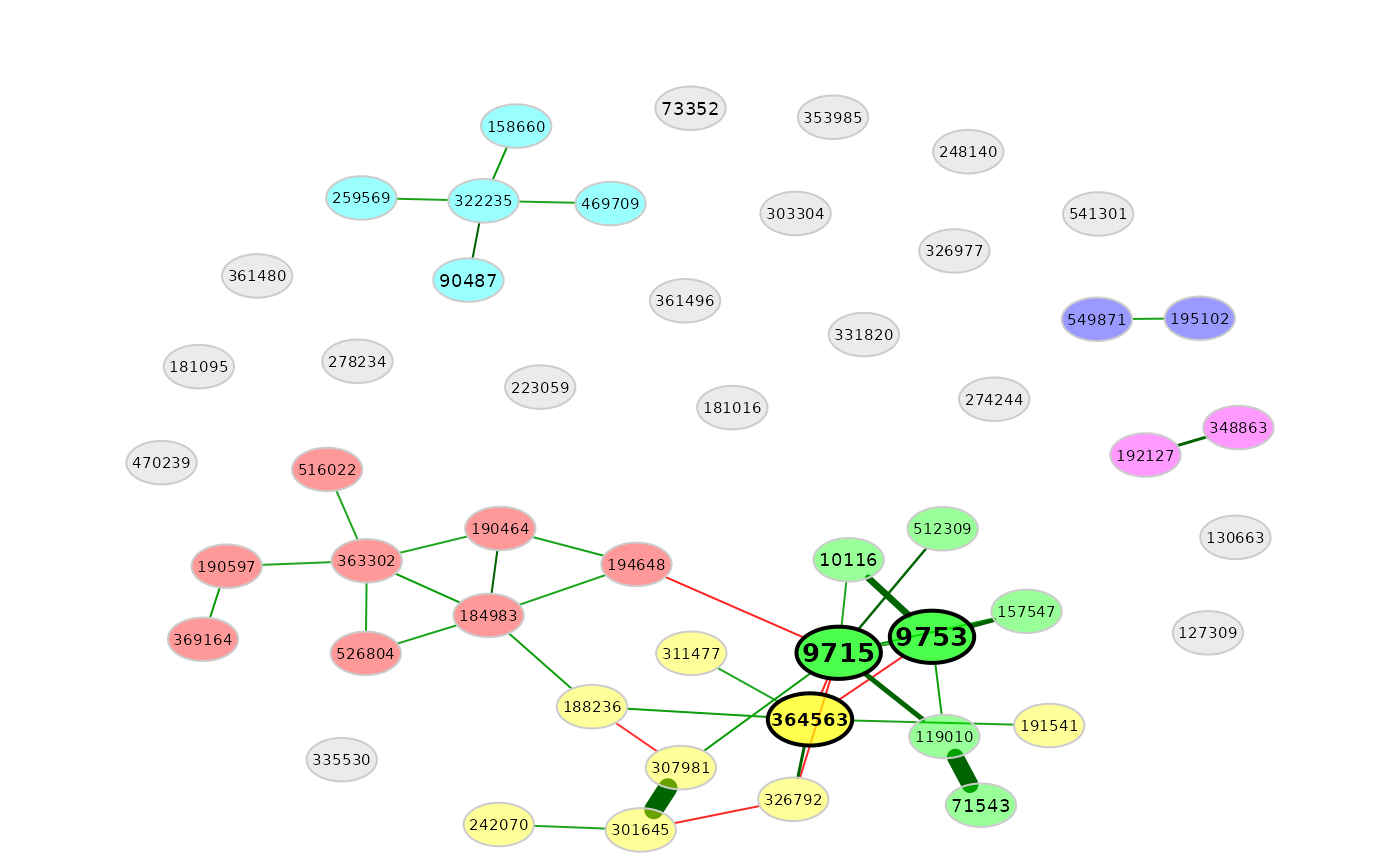
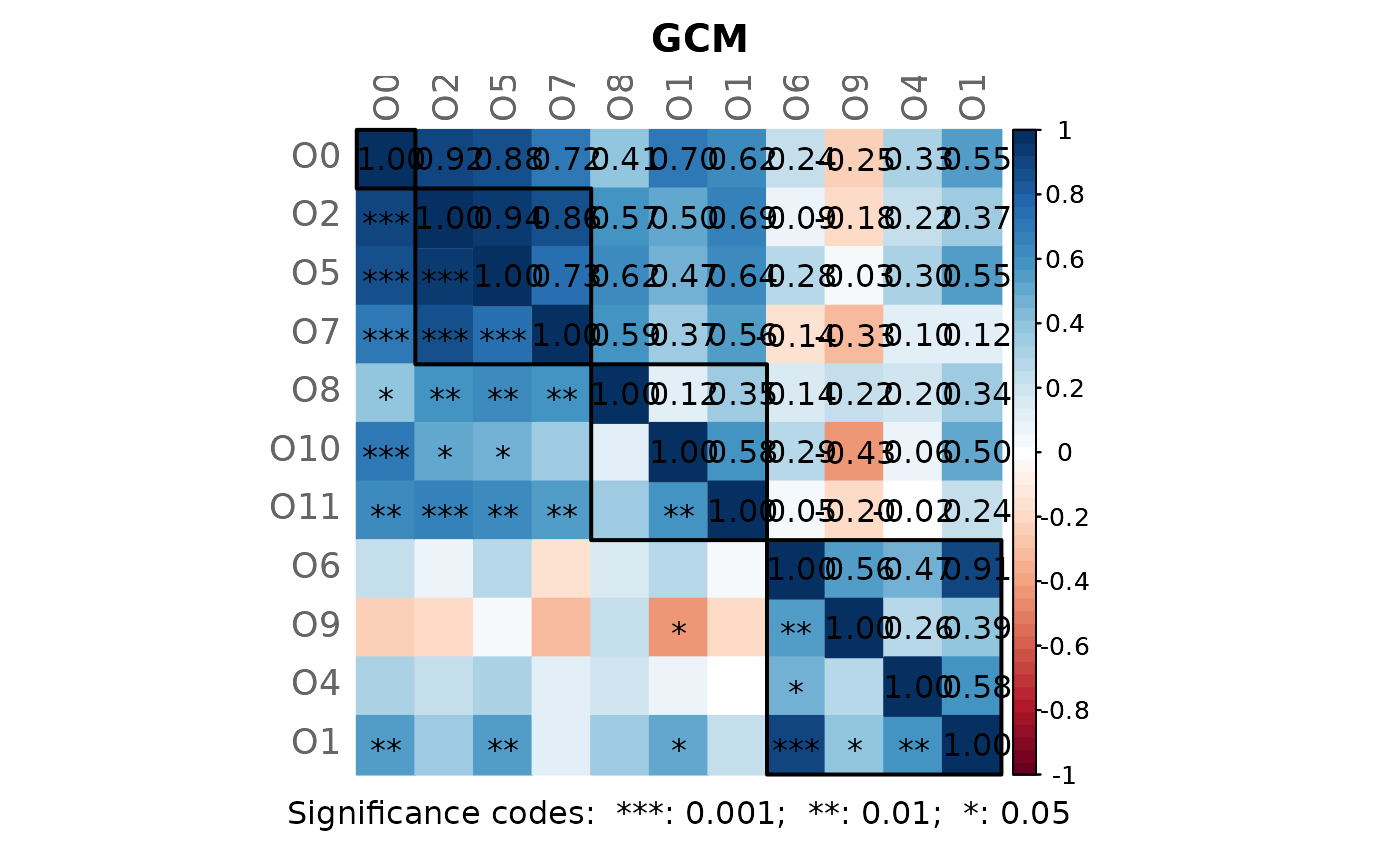 # Network plot (see ?plot.microNetProps for details)
plot(props1)
 #----------------------------------------------------------------------------
# Same network as before but on genus level and without taxa filtering
amgut.genus.phy <- phyloseq::tax_glom(amgut2.filt.phy, taxrank = "Rank6")
dim(phyloseq::otu_table(amgut.genus.phy))
#> [1] 43 296
# Rename taxonomy table and make Rank6 (genus) unique
amgut.genus.renamed <- renameTaxa(amgut.genus.phy, pat = "<name>",
substPat = "<name>_<subst_name>(<subst_R>)",
numDupli = "Rank6")
#> Column 7 contains NAs only and is ignored.
net_genus <- netConstruct(amgut.genus.renamed,
taxRank = "Rank6",
measure = "spieceasi",
measurePar = list(method = "mb",
pulsar.params = list(rep.num = 10),
symBetaMode = "ave"),
filtSamp = "totalReads",
filtSampPar = list(totalReads = 1000),
sparsMethod = "none",
normMethod = "none",
verbose = 3)
#> Checking input arguments ...
#> Done.
#> Data filtering ...
#> 35 samples removed.
#> 43 taxa and 261 samples remaining.
#>
#> Calculate 'spieceasi' associations ...
#>
#> Applying data transformations...
#> Selecting model with pulsar using stars...
#> Fitting final estimate with mb...
#> done
#> Done.
# Network analysis
props_genus <- netAnalyze(net_genus, clustMethod = "cluster_fast_greedy")
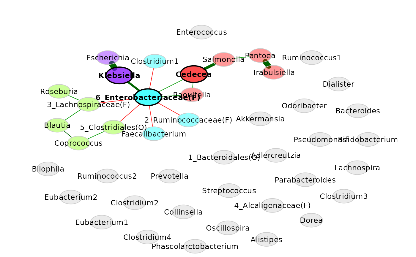
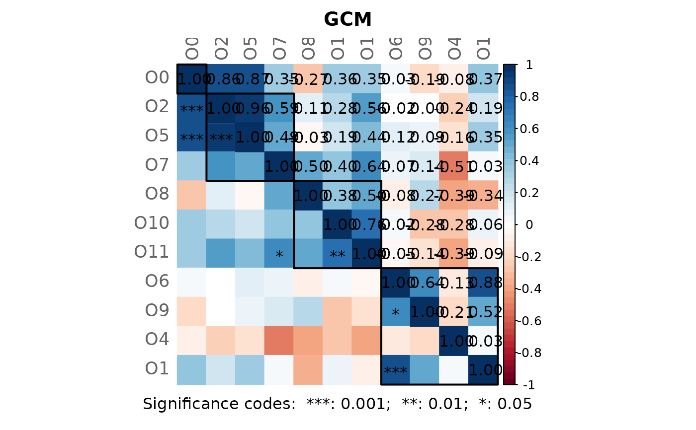 # Network plot (with some modifications)
plot(props_genus,
shortenLabels = "none",
labelScale = FALSE,
cexLabels = 0.8)
 #----------------------------------------------------------------------------
# Single network with the following specifications:
# - Association measure: Pearson correlation
# - Taxa filtering: Keep the 50 taxa with highest frequency
# - Sample filtering: Keep samples with a total number of reads of at least
# 1000 and with at least 10 taxa with a non-zero count
# - Zero replacement: A pseudo count of 0.5 is added to all counts
# - Normalization: clr transformation
# - Sparsification: Threshold = 0.3
# (an edge exists between taxa with an estimated association >= 0.3)
net2 <- netConstruct(amgut2.filt.phy,
measure = "pearson",
filtTax = "highestFreq",
filtTaxPar = list(highestFreq = 50),
filtSamp = c("numbTaxa", "totalReads"),
filtSampPar = list(totalReads = 1000, numbTaxa = 10),
zeroMethod = "pseudo",
zeroPar = list(pseudocount = 0.5),
normMethod = "clr",
sparsMethod = "threshold",
thresh = 0.3,
verbose = 3)
#> Checking input arguments ...
#> Done.
#> Data filtering ...
#> 35 samples removed.
#> 88 taxa removed.
#> 50 taxa and 261 samples remaining.
#>
#> Zero treatment:
#> Pseudo count of 0.5 added.
#>
#> Normalization:
#> Execute clr(){SpiecEasi} ...
#> Done.
#>
#> Calculate 'pearson' associations ...
#> Done.
#>
#> Sparsify associations via 'threshold' ...
#> Done.
# Network analysis
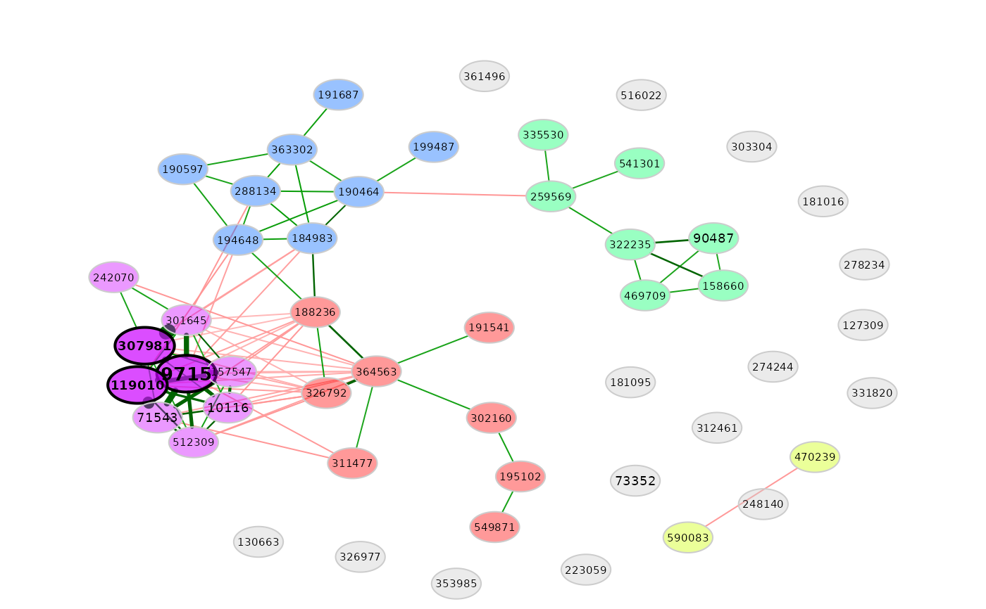
props2 <- netAnalyze(net2, clustMethod = "cluster_fast_greedy")
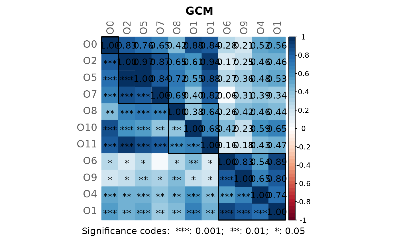 plot(props2)
 #----------------------------------------------------------------------------
# Example of using the argument "assoBoot"
# This functionality is useful for splitting up a large number of bootstrap
# replicates and run the bootstrapping procedure iteratively.
niter <- 5
nboot <- 1000
# Overall number of bootstrap replicates: 5000
# Use a different seed for each iteration
seeds <- sample.int(1e8, size = niter)
# List where all bootstrap association matrices are stored
assoList <- list()
for (i in 1:niter) {
# assoBoot is set to TRUE to return the bootstrap association matrices
net <- netConstruct(amgut1.filt,
filtTax = "highestFreq",
filtTaxPar = list(highestFreq = 50),
filtSamp = "totalReads",
filtSampPar = list(totalReads = 0),
measure = "pearson",
normMethod = "clr",
zeroMethod = "pseudoZO",
sparsMethod = "bootstrap",
cores = 1,
nboot = nboot,
assoBoot = TRUE,
verbose = 1, # Set to 2 for progress bar
seed = seeds[i])
assoList[(1:nboot) + (i - 1) * nboot] <- net$assoBoot1
}
#> Data filtering ...
#> 50 taxa and 289 samples remaining.
#>
#> Attaching package: ‘gtools’
#> The following objects are masked from ‘package:LaplacesDemon’:
#>
#> ddirichlet, logit, rdirichlet
#> The following object is masked from ‘package:permute’:
#>
#> permute
#> Data filtering ...
#> 50 taxa and 289 samples remaining.
#> Data filtering ...
#> 50 taxa and 289 samples remaining.
#> Data filtering ...
#> 50 taxa and 289 samples remaining.
#> Data filtering ...
#> 50 taxa and 289 samples remaining.
# Construct the actual network with all 5000 bootstrap association matrices
net_final <- netConstruct(amgut1.filt,
filtTax = "highestFreq",
filtTaxPar = list(highestFreq = 50),
filtSamp = "totalReads",
filtSampPar = list(totalReads = 0),
measure = "pearson",
normMethod = "clr",
zeroMethod = "pseudoZO",
sparsMethod = "bootstrap",
cores = 1,
nboot = nboot * niter,
assoBoot = assoList,
verbose = 1) # Set to 2 for progress bar
#> Data filtering ...
#> 50 taxa and 289 samples remaining.
# Network analysis
props <- netAnalyze(net_final, clustMethod = "cluster_fast_greedy")
 # Network plot
plot(props)
 #----------------------------------------------------------------------------
knitr::opts_chunk$set(fig.width = 16, fig.height = 8)
#----------------------------------------------------------------------------
# Constructing and analyzing two networks
# - A random group variable is used for splitting the data into two groups
set.seed(123456)
group <- sample(1:2, nrow(amgut1.filt), replace = TRUE)
# Option 1: Use the count matrix and group vector as input:
net3 <- netConstruct(amgut1.filt,
group = group,
measure = "pearson",
filtTax = "highestVar",
filtTaxPar = list(highestVar = 50),
filtSamp = "totalReads",
filtSampPar = list(totalReads = 1000),
zeroMethod = "multRepl",
normMethod = "clr",
sparsMethod = "t-test")
#> Checking input arguments ...
#> Done.
#> Data filtering ...
#> 77 taxa removed.
#> 50 taxa and 289 samples remaining.
#>
#> Zero treatment:
#> Execute multRepl() ...
#> Done.
#>
#> Normalization:
#> Execute clr(){SpiecEasi} ...
#> Done.
#>
#> Calculate 'pearson' associations ...
#> Done.
#>
#> Calculate associations in group 2 ...
#> Done.
#>
#> Sparsify associations via 't-test' ...
#>
#> Adjust for multiple testing via 'adaptBH' ...
#> Done.
#> Done.
#>
#> Sparsify associations in group 2 ...
#>
#> Adjust for multiple testing via 'adaptBH' ...
#> Done.
#> Done.
# Option 2: Pass the count matrix of group 1 to 'data'
# and that of group 2 to 'data2'
# Note: Argument 'jointPrepro' is set to FALSE by default (the data sets
# are filtered separately and the intersect of filtered taxa is kept,
# which leads to less than 50 taxa in this example).
amgut1 <- amgut1.filt[group == 1, ]
amgut2 <- amgut1.filt[group == 2, ]
net3 <- netConstruct(data = amgut1,
data2 = amgut2,
measure = "pearson",
filtTax = "highestVar",
filtTaxPar = list(highestVar = 50),
filtSamp = "totalReads",
filtSampPar = list(totalReads = 1000),
zeroMethod = "multRepl",
normMethod = "clr",
sparsMethod = "t-test")
#> Checking input arguments ...
#> Done.
#> Data filtering ...
#> 85 taxa removed in each data set.
#> 42 taxa and 138 samples remaining in group 1.
#> 42 taxa and 151 samples remaining in group 2.
#>
#> Zero treatment in group 1:
#> Execute multRepl() ...
#> Done.
#>
#> Zero treatment in group 2:
#> Execute multRepl() ...
#> Done.
#>
#> Normalization in group 1:
#> Execute clr(){SpiecEasi} ...
#> Done.
#>
#> Normalization in group 2:
#> Execute clr(){SpiecEasi} ...
#> Done.
#>
#> Calculate 'pearson' associations ...
#> Done.
#>
#> Calculate associations in group 2 ...
#> Done.
#>
#> Sparsify associations via 't-test' ...
#>
#> Adjust for multiple testing via 'adaptBH' ...
#> Done.
#> Done.
#>
#> Sparsify associations in group 2 ...
#>
#> Adjust for multiple testing via 'adaptBH' ...
#> Done.
#> Done.
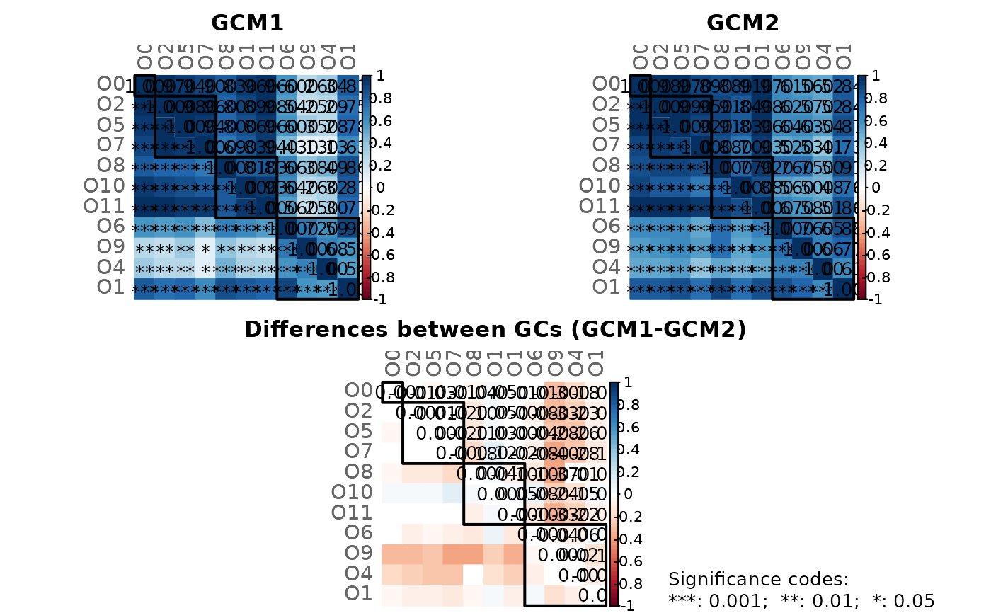
# Network analysis
# Note: Please zoom into the GCM plot or open a new window using:
# x11(width = 10, height = 10)
props3 <- netAnalyze(net3, clustMethod = "cluster_fast_greedy")
#----------------------------------------------------------------------------
knitr::opts_chunk$set(fig.width = 16, fig.height = 8)
#----------------------------------------------------------------------------
# Constructing and analyzing two networks
# - A random group variable is used for splitting the data into two groups
set.seed(123456)
group <- sample(1:2, nrow(amgut1.filt), replace = TRUE)
# Option 1: Use the count matrix and group vector as input:
net3 <- netConstruct(amgut1.filt,
group = group,
measure = "pearson",
filtTax = "highestVar",
filtTaxPar = list(highestVar = 50),
filtSamp = "totalReads",
filtSampPar = list(totalReads = 1000),
zeroMethod = "multRepl",
normMethod = "clr",
sparsMethod = "t-test")
#> Checking input arguments ...
#> Done.
#> Data filtering ...
#> 77 taxa removed.
#> 50 taxa and 289 samples remaining.
#>
#> Zero treatment:
#> Execute multRepl() ...
#> Done.
#>
#> Normalization:
#> Execute clr(){SpiecEasi} ...
#> Done.
#>
#> Calculate 'pearson' associations ...
#> Done.
#>
#> Calculate associations in group 2 ...
#> Done.
#>
#> Sparsify associations via 't-test' ...
#>
#> Adjust for multiple testing via 'adaptBH' ...
#> Done.
#> Done.
#>
#> Sparsify associations in group 2 ...
#>
#> Adjust for multiple testing via 'adaptBH' ...
#> Done.
#> Done.
# Option 2: Pass the count matrix of group 1 to 'data'
# and that of group 2 to 'data2'
# Note: Argument 'jointPrepro' is set to FALSE by default (the data sets
# are filtered separately and the intersect of filtered taxa is kept,
# which leads to less than 50 taxa in this example).
amgut1 <- amgut1.filt[group == 1, ]
amgut2 <- amgut1.filt[group == 2, ]
net3 <- netConstruct(data = amgut1,
data2 = amgut2,
measure = "pearson",
filtTax = "highestVar",
filtTaxPar = list(highestVar = 50),
filtSamp = "totalReads",
filtSampPar = list(totalReads = 1000),
zeroMethod = "multRepl",
normMethod = "clr",
sparsMethod = "t-test")
#> Checking input arguments ...
#> Done.
#> Data filtering ...
#> 85 taxa removed in each data set.
#> 42 taxa and 138 samples remaining in group 1.
#> 42 taxa and 151 samples remaining in group 2.
#>
#> Zero treatment in group 1:
#> Execute multRepl() ...
#> Done.
#>
#> Zero treatment in group 2:
#> Execute multRepl() ...
#> Done.
#>
#> Normalization in group 1:
#> Execute clr(){SpiecEasi} ...
#> Done.
#>
#> Normalization in group 2:
#> Execute clr(){SpiecEasi} ...
#> Done.
#>
#> Calculate 'pearson' associations ...
#> Done.
#>
#> Calculate associations in group 2 ...
#> Done.
#>
#> Sparsify associations via 't-test' ...
#>
#> Adjust for multiple testing via 'adaptBH' ...
#> Done.
#> Done.
#>
#> Sparsify associations in group 2 ...
#>
#> Adjust for multiple testing via 'adaptBH' ...
#> Done.
#> Done.
# Network analysis
# Note: Please zoom into the GCM plot or open a new window using:
# x11(width = 10, height = 10)
props3 <- netAnalyze(net3, clustMethod = "cluster_fast_greedy")
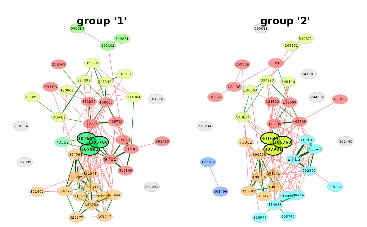
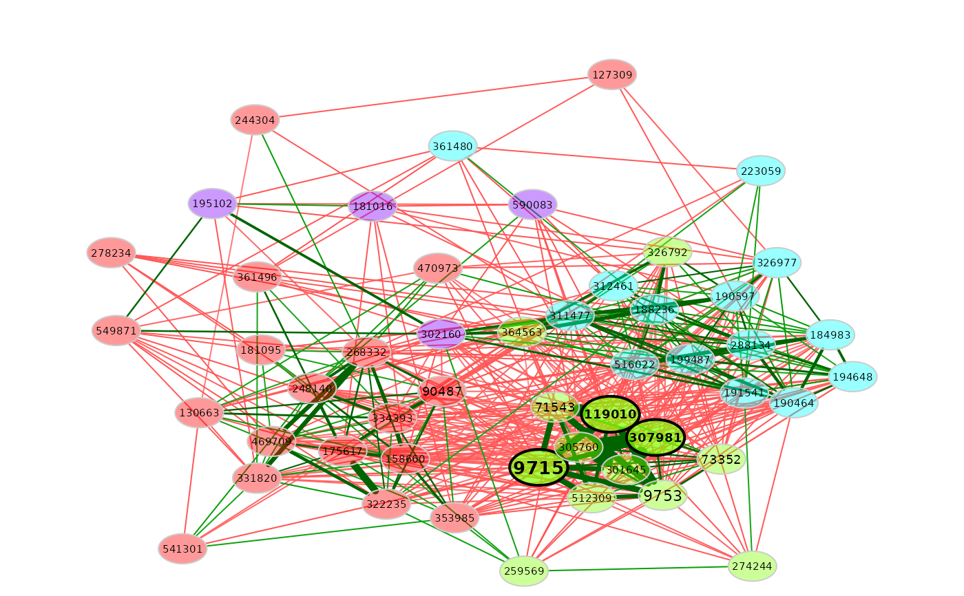
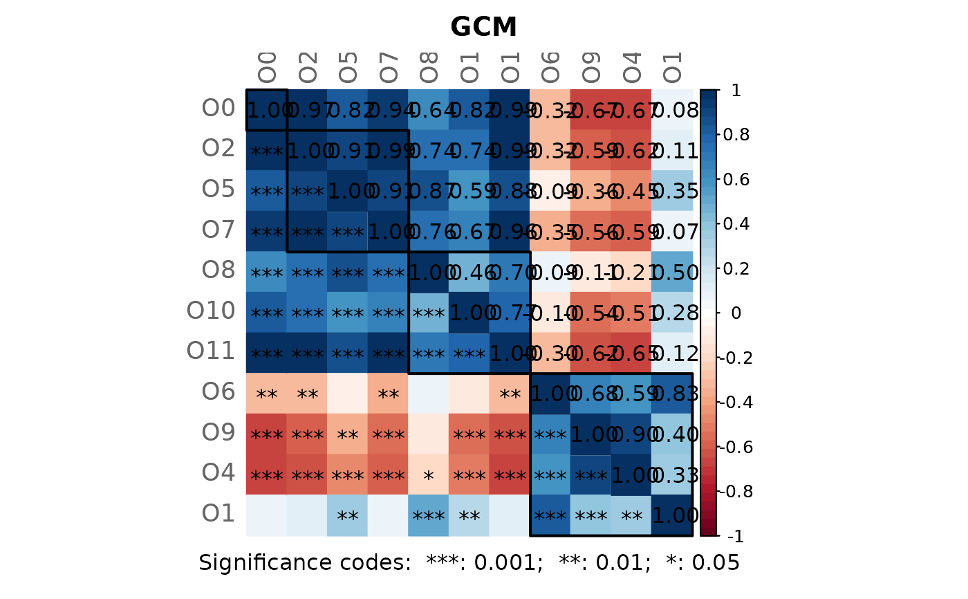 # Network plot (same layout is used in both groups)
plot(props3, sameLayout = TRUE)
 # The two networks can be compared with NetCoMi's function netCompare().
